Microsoft Excel – Change Row Color Based On a Cell Value
Sometimes we need automatic colorisation of the rows based on the value of a cell. Its not only save lot of time as well as simplify identification of records based on the colors. Thanks to excel conditional formating that allow you to do. Formatting cell based on the condition is easy but formating entire row or column is little tricky.
To Do ->
Select the area you want to cover for formatting. You can select entire workbook if you want to cover complete all cell and columns.
Go to Format Menu -> Conditional Formatting
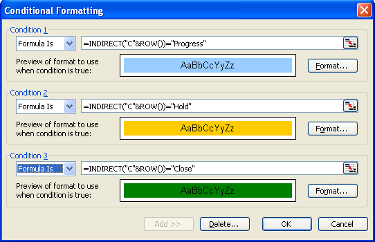
See the above figure, you will notice INDIRECT function. The INDIRECT function used to create cell or range reference while formula evaluated. The function allows you to put the address of another cell within a cell, and get data from the the other cell by referencing the first cell.? ?
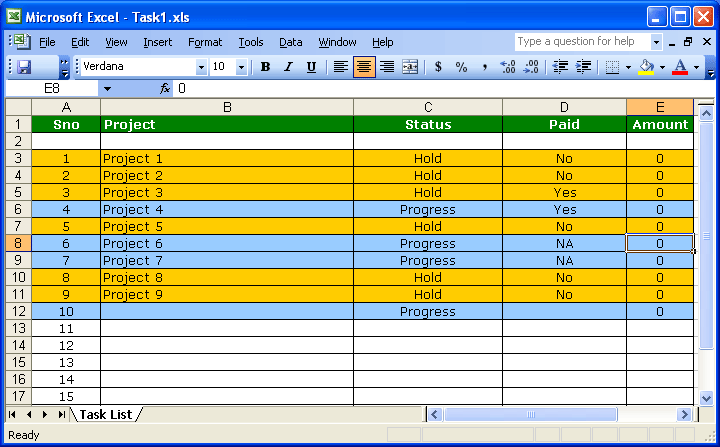
The condition check column C in each selected row and change formatting according to specification.


Fantastic…. easy to follow steps and the result is very much as expected
Thanks for the help! I have an additional condition to add and am not sure of the formatting or if it can be done. I would like to add the 3rd condition and another row, that if the column H has a date in it the column goes back to no color even with one of the first 2 conditions met. Is that possible? Hope I explained that correctly.
Thanks
Thank you very much. I’ve been looking for this for 2 hours. This has been a major help 🙂
WOW! ITS SUPERB!
EASY TO UNDERSTAND. I HOPE I CAN LEARN MORE ON EXCEL.
thanks….for this posting 🙂
Spent an hour on other sites trying their directions… got it really easy with yours… thanks!!!!!